Doctoral school course: an introduction to R
Block 1: : R, R Studio, programmation basics and random variables
R and R Studio
What is it ?
A first quote from wikipedia:
R is a programming language for statistical computing and data visualization. It has been adopted in the fields of data mining, bioinformatics and data analysis. The core R language is augmented by a large number of extension packages, containing reusable code, documentation, and sample data. R software is open-source and free software. It is licensed by the GNU Project and available under the GNU General Public License. It is written primarily in C, Fortran, and R itself. Precompiled executables are provided for various operating systems.
and a second one:
RStudio IDE (or RStudio) is an integrated development environment for R, a programming language for statistical computing and graphics. It is available in two formats: RStudio Desktop is a regular desktop application while RStudio Server runs on a remote server and allows accessing RStudio using a web browser. The RStudio IDE is a product of Posit PBC (formerly RStudio PBC, formerly RStudio Inc.).
In this tutorial we will be using the R Studio development environment for R. You need to download R and then download R Studio as explained here.
Where can I learn R ?
This tutorial R for data sciences is a quite good one.
Nevertheless, I will use a slightly different path here by beginning to learn R without installing extra packages, at least in a first time.
The generative artificial intelligence chatbots can also help you a lot… once you have learned the basics.
Open RStudio !
Once R and RStudio have been installed on your machine, you can start RStudio.
R Studio windows
When RStudio is launched, the screen is divided into three main areas.
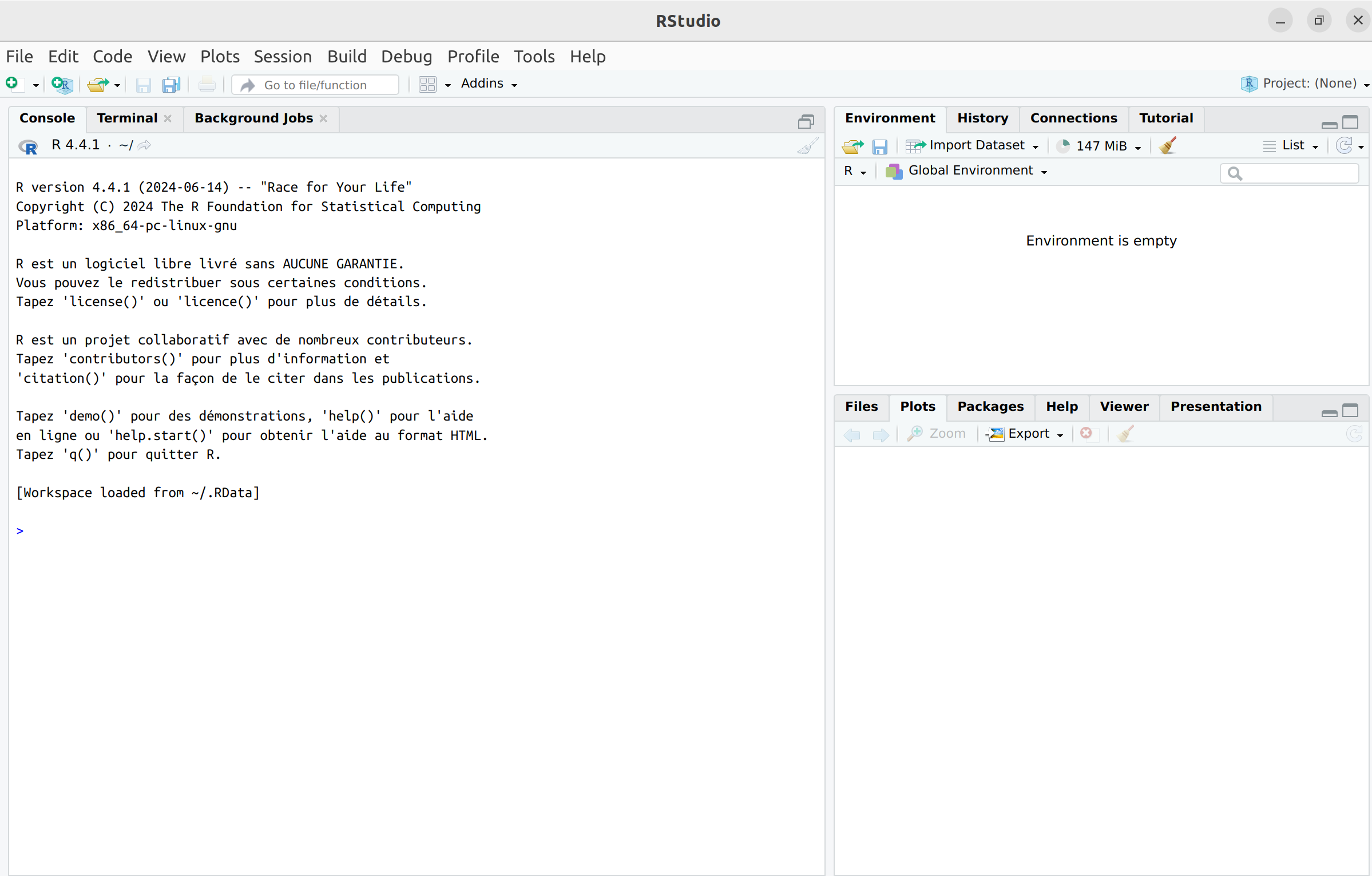
The left area is called the Console, where you can
see the version of R loaded by RStudio upon startup. After the
introductory text, the line starts with > –this is the
command prompt. RStudio is now ready to receive your first command. You
can use R as a calculator. For example, type:
2 + 3## [1] 5Press Enter, and the result will appear in the Console.
At the top right, in the Environment tab, you can see a list of objects and functions created as you work. Additionally, the History tab provides access to your command history.
At the bottom right, you will find several tabs:
- Files: Displays the contents of your working directory.
- Plots: Displays the plots you create.
- Packages: Lists the installed packages, allowing you to load, update, or install new ones (see the dedicated section).
- Help: Provides access to online help.
You can customize the configuration of RStudio tabs by going to View-> Panes -> Pane Layout.
RStudio document types
By navigating to File -> New File or clicking the arrow next to the New File icon (at the top left), RStudio offers a variety of document types. Note that RStudio can also be used for other languages like Python, C++, and more.

Here, we will focus only on a few file types that will be used later. When you select a file type, a fourth window opens in the top-left area of the RStudio interface.
To create an R script, simply select R Script. This
script can be saved at any time as a file with the extension
.R (e.g., myScript.R) in the current directory
by clicking on the floppy disk icon or through File ->
Save. You can reopen it at any time via the menu File
-> Open File…, by clicking the folder icon, or by
double-clicking the myScript.R file. It is also possible to
execute a script directly from the console using the command
source("myScript.R").
You can create a document (report, slides, etc.) using
RMarkdown by selecting R Markdown.
This allows you to edit documents in formats such as PDF or HTML,
including R commands, outputs, and plots. The new document will be saved
with the .Rmd extension. During creation, you need to
specify the desired final document type (HTML, PDF, presentation, etc.)
and the document details (title and author).
We will explore the possibilities of RMarkdown and the main commands for drafting a report in more detail later.
Environment and Working Directory
Working Directory
To manage data retrieval, script saving, and results storage, it is
important to know the working directory—this is the default directory
where various results will be saved. You can check the current working
directory using the command: getwd().
To change the working directory, you can use the setwd()
command in the Console. Note that R only recognizes the /
character for specifying directory paths, even on Windows.
Alternatively, you can navigate to Session -> Set Working
Directory -> Choose Directory.
R Help System
It is normal to forget or be unsure about a function’s arguments or their names. At any time, you can access R’s built-in help system. For example, to get help for the plot function, you can use:
help(plot)or the shortcut:
?plotBoth commands display a help page (in English) with a description of the function, its parameters, output, examples, and more. These help pages contain detailed information but can sometimes be difficult to read.
In RStudio, help pages will open by default in the bottom-right pane under the Help tab. Clicking the house icon will take you to the home page of the help system. You can also search directly for a function’s name using the search bar in the Help tab.
A gentle introduction through an example of dataset
There is a lot of data sets that are already available in R without installing extra package or downloading data files. This is particularly useful when you want to test statistical methods or commands. To have an overview, type into the R console:
??datasets
library(help="datasets")
Note that the dataset documentation opens in a new tab.
1. The beavers dataset
Let us play with one of these datasets to learn some programmation basics. I choose, quite at random for this tutorial the dataset about the body temperature of two beavers. Type into the console:
data(beavers)Note that the two variables beaver1 and
beaver2 appear into the environment panel. We use
the class() command to find out the class of an object and
str() to find out the nature of the elements making up the
object:
class(beaver1)## [1] "data.frame"str(beaver1)## 'data.frame': 114 obs. of 4 variables:
## $ day : num 346 346 346 346 346 346 346 346 346 346 ...
## $ time : num 840 850 900 910 920 930 940 950 1000 1010 ...
## $ temp : num 36.3 36.3 36.4 36.4 36.5 ...
## $ activ: num 0 0 0 0 0 0 0 0 0 0 ...Thus, the class of the object beaver1 is
data.frame. In R, a data.frame is a data
structure used to store tabular data in rows and columns, much like a
spreadsheet or a SQL table. It is one of the most commonly used classes
in R for handling and analyzing structured data. A
data.frame object has the following characteristics:
- Tabular Format:
- A data.frame organizes data in rows and columns.
- Each column represents a variable, and each row represents an observation.
- Heterogeneous Columns:
- Columns can contain different data types (e.g., numeric, character, factor, logical).
- All elements within a column must be of the same data type.
- Homogeneous Rows: Each row is treated as a single observation and can combine elements from all columns.
- Column Names: Each column must have a name, which can be used for accessing or referencing it.
- Row Names (Optional): By default, data.frame assigns row names as integers, but custom row names can also be set.
- Indexing and Access:
- Columns can be accessed using $, column names, or by numeric indexing.
- Rows and columns can be accessed using [row, column] indexing.
Note that all the variables of the data frame beaver1
have num as type, meaning that these variables are numerics
so that it should make sens, for instance, to compute the mean of each
column. There is always a default type, but it is not necessarily the
most appropriate one, and you need to be careful because this can have
consequences. There is in fact a hierarchy of types:
NULL < raw < logical < integer < double < complex < character < list < expression
The output type is determined from the highest type of the components
in this hierarchy (where double is identical to
numeric). We will not use the raw and
complex types in this tutorial but we should see the other
types.
x=c(TRUE,1,3.24,"abc")
class(x)
## [1] "character"All vector entries have been assigned the type
character, the highest one.
Let us check if the types are the good one by looking at the
documention associated to the dataset, opening in the help
panel:
?beaversFor the variable day and time, the type
num is questionable but might be accepted, for
temp, it seems quite appropriate but for
activ, it does not seem right since it is an indicator of
activity outside the retreat. It should be a factorial variable
(also called categorical or qualitative).
Go to the next tab !
2. About factorial variables
You can change the type of a variable to a factorial variable as follows:
beaver1$activ<-as.factor(beaver1$activ)Let us comment a little bit this code line. At first, to access the
variables of the dataset beaver1, we used the
$ operator.
Then, we used the <- operator to asign to the
variable beaver$activ the new value
as.factor(beaver1$activ). In general, an object can be
stored in a variable (e.g., a) using
a <- ... or a = ..., these two ways of
asignement being often interchageable but not always. The good pratice
in R is the following one:
- Use
<-for assignment in your R scripts to adhere to R programming norms. - Use
=strictly for assigning values to function arguments (we will see how to write functions later…).
Let us look at what have changed:
class(beaver1$activ)## [1] "factor"The variable beaver1$activ is now a factorial variable
having levels (or categories or factors):
levels(beaver1$activ)## [1] "0" "1"You can change these levels:
levels(beaver1$activ)<-c("Not activ", "Activ")
levels(beaver1$activ)
## [1] "Not activ" "Activ"When belonging to the right class, the R base command
plot produces an appropriate graphic adapted to the type of
the variable. You can experiment that:
par(mfrow=c(1,2))
plot(beaver1$activ)
plot(as.numeric(beaver1$activ))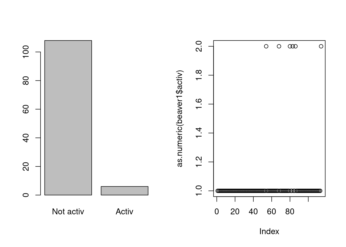
When we asign to beaver$activ the numerical type, R
produces a x-y-plot with the valuers 0 and 1 for the y-axis and for the
x-axis, the rank of the plotted value. But when stored with the right
type, R produces a barplot for the categorical variable and this is
quite appropriate.
Above, we have used the par(mfrow=c(1,2)) command. This
command is used to configure the graphical layout for plotting multiple
figures on a single plotting device:
- The
par()function is used to set or query graphical parameters in R. - The
mfrowargument inpar()specifies how the plotting area should be divided into a grid of rows and columns for displaying multiple plots. Here,c(1,2)means 1 row and 2 columns, i.e., the plotting area will be divided into two side-by-side panels. To reset, usepar(mfrow=c(1,1))or restart the plotting device withdev.off()(without any parameter).
When you produce a graphic, you can modify many parameters (title, color, line thickness, etc.). I invite you to try as many as you can. Here is an example:
plot(beaver1$activ,col=c("red","blue"),
     main="A barplot for beaver1")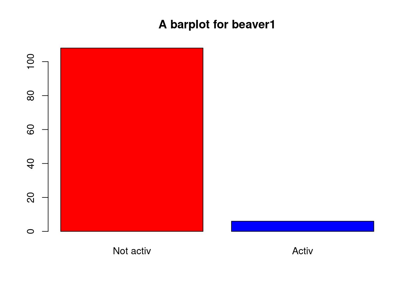
What can we do with an univariate qualitative variable ? You can get the count of the levels as follows:
table(beaver1$activ)##
## Not activ Activ
## 108 6To obtain the percentages, it is as follows:
prop.table(table(beaver1$activ))##
## Not activ Activ
## 0.94736842 0.05263158Note that it actually is prop.table of the output of
table, and not just prop.table of the
considered variable. One way of representing this kind of data, which is
often considered bad (but this is debatable), is to draw a pie
chart:
par(mfrow=c(1,2))
pie(table(beaver1$activ))
plot(beaver1$activ)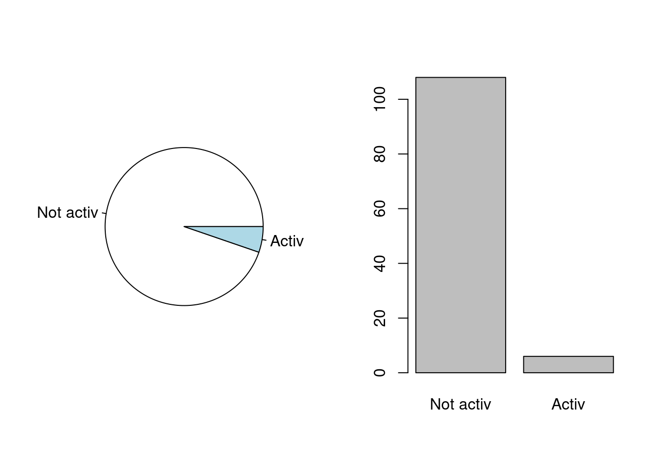
Do you find one chart more meaningful than the other?
There is another type of categorical variable (a sub-category), when there is a natural order in between the levels. For example:
my_vector<-c("bad","good","good","fair","bad","fair","bad")
my_vector<-as.ordered(my_vector)
my_vector
## [1] bad good good fair bad fair bad
## Levels: bad < fair < goodHere we have been lucky with the lexical order. But what if we want a specific order?
my_vector<-ordered(my_vector,levels=c("fair","good","bad"))
my_vector
## [1] bad good good fair bad fair bad
## Levels: fair < good < badGo to the next tab !
3. Operations on numerical variables (and scalar operations)
In the data frame beaver1, are the numerical variables
day and time. Let’s take a look:
beaver1$day## [1] 346 346 346 346 346 346 346 346 346 346 346 346 346 346 346 346 346 346 346 346 346 346 346
## [24] 346 346 346 346 346 346 346 346 346 346 346 346 346 346 346 346 346 346 346 346 346 346 346
## [47] 346 346 346 346 346 346 346 346 346 346 346 346 346 346 346 346 346 346 346 346 346 346 346
## [70] 346 346 346 346 346 346 346 346 346 346 346 346 346 346 346 346 346 346 346 346 346 346 347
## [93] 347 347 347 347 347 347 347 347 347 347 347 347 347 347 347 347 347 347 347 347 347 347There is therefore 2 different days: we can have this
information thanks to the unique function, which returns an
object of the same type of its argument, but with the duplicate elements
or rows removed:
unique(beaver1$day)## [1] 346 347Let us take a look at the time variable:
beaver1$time## [1] 840 850 900 910 920 930 940 950 1000 1010 1020 1030 1040 1050 1100 1110 1120 1130 1140
## [20] 1150 1200 1210 1220 1230 1240 1250 1300 1310 1320 1330 1340 1350 1400 1410 1420 1430 1440 1450
## [39] 1500 1510 1520 1530 1540 1550 1600 1610 1620 1630 1640 1650 1700 1710 1720 1730 1740 1750 1800
## [58] 1810 1820 1830 1840 1850 1900 1910 1920 1930 1940 1950 2000 2010 2020 2030 2040 2050 2100 2110
## [77] 2120 2130 2140 2150 2200 2210 2230 2240 2250 2300 2310 2320 2330 2340 2350 0 10 20 30
## [96] 40 50 100 110 120 130 140 150 200 210 220 230 240 250 300 310 320 330 340We see, at a first look, that the body temperature was measured every 10 minutes, most of the times. We can obtain the vector of the differences the folowing way:
diff(beaver1$time)## [1] 10 50 10 10 10 10 10 50 10 10 10 10 10 50 10
## [16] 10 10 10 10 50 10 10 10 10 10 50 10 10 10 10
## [31] 10 50 10 10 10 10 10 50 10 10 10 10 10 50 10
## [46] 10 10 10 10 50 10 10 10 10 10 50 10 10 10 10
## [61] 10 50 10 10 10 10 10 50 10 10 10 10 10 50 10
## [76] 10 10 10 10 50 10 20 10 10 50 10 10 10 10 10
## [91] -2350 10 10 10 10 10 50 10 10 10 10 10 50 10 10
## [106] 10 10 10 50 10 10 10 10unique(diff(beaver1$time))## [1] 10 50 20 -2350So this ever 10, 20 or 50 minutes, but most often than not, every 10 minutes:
table(diff(beaver1$time))##
## -2350 10 20 50
## 1 93 1 18The \(-2350\) is due to the change of day.
To learn how to manipulate quantitative variables, let’s try to
obtain, from the vectors day and time, the
time that has elapsed since the first measurement, in hours:
hours<-24*(beaver1$day-beaver1$day[1])+floor(beaver1$time/100)+(beaver1$time-100*floor(beaver1$time/100))/60There is a lot in this formula. At first, we have condidered the days
stored in beaver1$day. The first entry of this numerical
vector is obtained thank to beaver1$day[1]:
beaver1$day[1]## [1] 346We then subtracted the number of the first day from the current day to obtain the number of days elapsed since the start of the experiment. For this, we type:
beaver1$day-beaver1$day[1]## [1] 0 0 0 0 0 0 0 0 0 0 0 0 0 0 0 0 0 0 0 0 0 0 0 0 0 0 0 0 0 0 0 0 0 0 0 0 0 0 0 0 0 0 0 0 0 0 0
## [48] 0 0 0 0 0 0 0 0 0 0 0 0 0 0 0 0 0 0 0 0 0 0 0 0 0 0 0 0 0 0 0 0 0 0 0 0 0 0 0 0 0 0 0 0 1 1 1
## [95] 1 1 1 1 1 1 1 1 1 1 1 1 1 1 1 1 1 1 1 1But not that in doing so, we susbtract to an object of dimension
length(beaver1$day), that is 114, a number (of length one).
But it works since R automatically recasts the scalar as an object of
the appropriate dimension, if possible. This is as convenient as it can
be bad, depending of what we really intend to do. It means that for
example \((y_1,y_2,y_3)-a\) is
understood as \((y_1,y_2,y_3)-(a,a,a)=(y_1-a,y_2-a,y_3-a)\).
We see in the above formula that we can add, substract, two numerical
vectors, and multiply and divide a numerical vector by a scalar. We also
used the floor function taking a single numeric argument x
and returning a numeric vector containing the largest integers not
greater than the corresponding elements of x:
floor(4.3)## [1] 4vect<-c(2.3,1,-4.6)
floor(vect)## [1] 2 1 -5Above, we have used the generic function c which
combines its arguments. It is a comon way to create small
vectors. From the help of R, ?c, we learn that all
arguments are coerced to a common type which is the type of the returned
value, and all attributes except names are removed. The output type is
the highest:
vect<-c(1.2,"hello",TRUE)
vect
## [1] "1.2" "hello" "TRUE"We see that all elements have be turned into the character type.
Let us go back to the numerical vectors hours that we
have just created by looking at its head, that is, its
first values:
head(hours)## [1] 8.666667 8.833333 9.000000 9.166667 9.333333 9.500000We can plot the temperature of the first beaver in function of the hour as follows:
plot(hours,beaver1$temp,main="Body temperature of beaver1",
     xlab="time (in hours)",
     ylab="temperature (in degrees Celsius)",
     pch=19)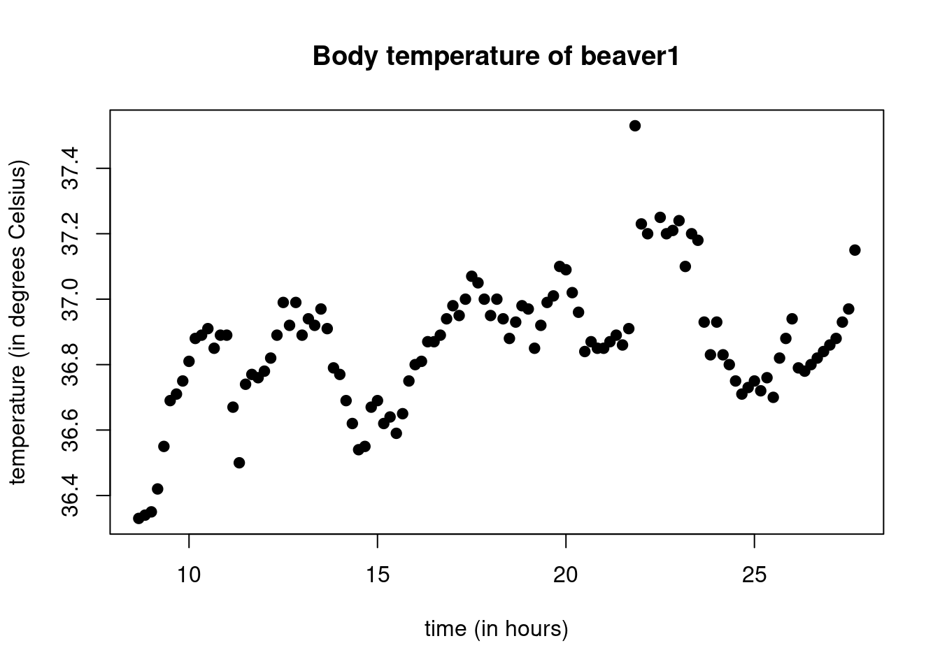
Above, we have used the plot function, providing it with
the x-axis vector (hours) and the y-axis vector
(beaver1$temp). We also used the argument main
to provide the main title, xlab for the label of the x-axis
and ylab for the label of the y-axis. The argument
pch allows to choose the type of points, there is quite a
lot of basic choices form 0 to 25.
Exercise: plot the body temperature of beaver1 in Farenheit, with square points colored in red.
Go to the next tab !
4. Basic one dimensional statistics and basic functions
What about the basic statistical characteristics of the body temperature of beaver1?
Mean and median
The mean body temperature of beaver1 is obtained through
temp1<-beaver1$temp
mean(temp1)
## [1] 36.86219Let us check this value by using the sum and
length functions:
sum(temp1)/length(temp1)## [1] 36.86219In statistics, we say that the mean is an indicator of
the central tendency of the distribution. Another widely used
indicator of central tendency is the median:
median(temp1)## [1] 36.87For this data set, the median is very close to the mean, but this is not always the case. However, it can be shown that the difference between the mean and the median cannot exceed one standard deviation.
Let us check that the median is indeed this one, which will help us
learn other basic R functions. To compute the median, we have to sort
the data, we use the sort function for this purpose:
sort(temp1)## [1] 36.33 36.34 36.35 36.42 36.50 36.54 36.55 36.55 36.59 36.62 36.62 36.64 36.65 36.67 36.67
## [16] 36.69 36.69 36.69 36.70 36.71 36.71 36.72 36.73 36.74 36.75 36.75 36.75 36.75 36.76 36.76
## [31] 36.77 36.77 36.78 36.78 36.79 36.79 36.80 36.80 36.80 36.81 36.81 36.82 36.82 36.82 36.83
## [46] 36.83 36.84 36.84 36.85 36.85 36.85 36.85 36.86 36.86 36.87 36.87 36.87 36.87 36.88 36.88
## [61] 36.88 36.88 36.89 36.89 36.89 36.89 36.89 36.89 36.89 36.91 36.91 36.91 36.92 36.92 36.92
## [76] 36.93 36.93 36.93 36.93 36.94 36.94 36.94 36.94 36.95 36.95 36.96 36.97 36.97 36.97 36.98
## [91] 36.98 36.99 36.99 36.99 37.00 37.00 37.00 37.01 37.02 37.05 37.07 37.09 37.10 37.10 37.15
## [106] 37.18 37.20 37.20 37.20 37.21 37.23 37.24 37.25 37.53There is 114 values so that the median is defined as the mean of the entries 57 and 58 of the sorted vector:
sort_temp1<-sort(temp1)
(sort_temp1[57]+sort_temp1[58])/2
## [1] 36.87As expected, this gives the same thing as the function
median. Recall that the median of a set of numbers is the
value separating the higher half from the lower half of a data sample.
It is the quantile of order \(1/2\):
\(50\%\) of the data are above the
median, and \(50\%\) below.
Let us, as an exercise, plot the values coloured according of wheter there are above or below the median. At first, we define a vector of colours
colour<-rep("blue",length=length(temp1))Now, when the value is above the median, we set the colour to
red:
colour[temp1>median(temp1)]="red"And then, we do the plot:
plot(hours,temp1,col=colour)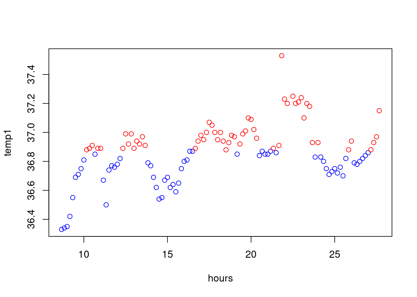
Let us now chantge the type of the points when this is above the mean:
my_pt<-rep(1,length=length(temp1))
my_pt[temp1>mean(temp1)]=19
plot(hours,temp1,col=colour,pch=my_pt)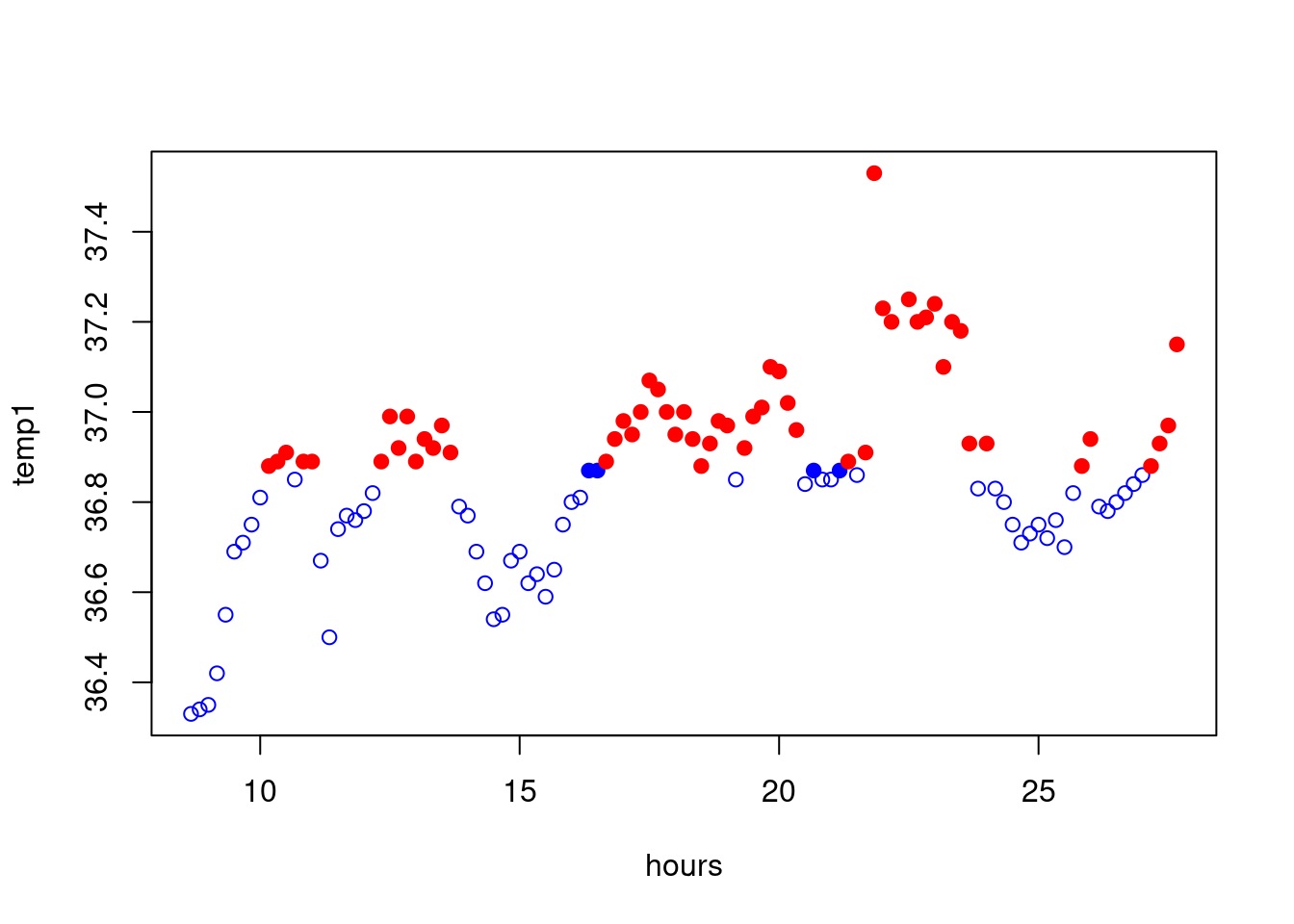
Other quantiles can be considered. The quantile of order \(\alpha\in(0,1)\) it the (a…) real such that
\(100\alpha\%\) of the data are below
this number. In R, we can compute all possible quantiles thanks to the
quantile function the following way:
quantile(temp1,probs = 0.5)## 50%
## 36.87This is the median. But we can also look at the first and third quartiles:
quantile(temp1,probs=c(0.25,0.75))## 25% 75%
## 36.7600 36.9575Exercise: Color the plot of the temperature according to the first and third quartiles.
A good way to visualize quantiles is with a whisker box or boxplot:
boxplot(temp1,main="Boxplot of the Body temperature of beaver1",
        ylab="Temperature (Celsius)")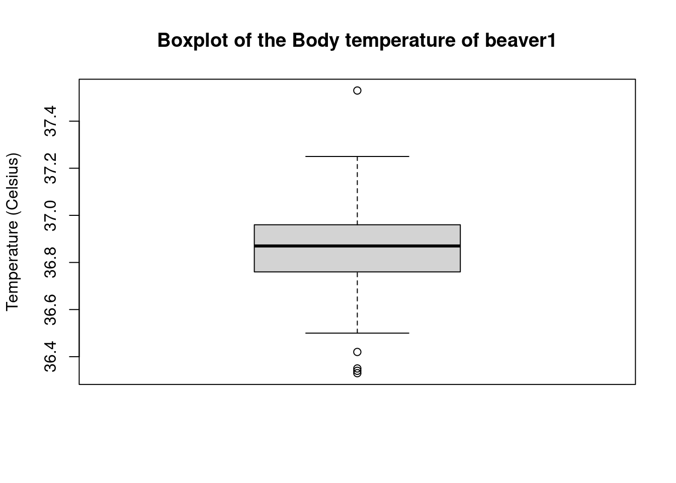
We see that the outliers, that is the values that lie beyond the whiskers, are ploted as points. Can we obtain these values ? In fact, we can always store a plot in a variable which contains the values (as a list here) used to obtain the graph:
bb<-boxplot(temp1)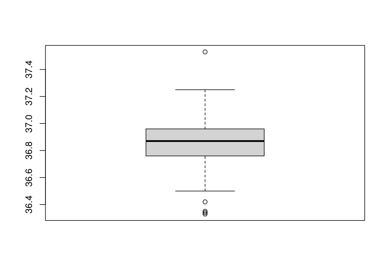
str(bb)## List of 6
## $ stats: num [1:5, 1] 36.5 36.8 36.9 37 37.2
## $ n : num 114
## $ conf : num [1:2, 1] 36.8 36.9
## $ out : num [1:5] 36.3 36.3 36.4 36.4 37.5
## $ group: num [1:5] 1 1 1 1 1
## $ names: chr "1"The variable bb$stats contains the extreme of the lower
whisker, the lower hinge, the median, the upper hinge and the extreme of
the upper whisker. The values that lie beyond the whisker are stored in
bb$out:
bb$out## [1] 36.33 36.34 36.35 36.42 37.53Another way to access the element of a liste is to use the double square brackets:
bb[[4]]## [1] 36.33 36.34 36.35 36.42 37.53Sometimes, it might be preferable to not draw the outliers, for this,
use the argument outline=F:
boxplot(temp1,outline=F)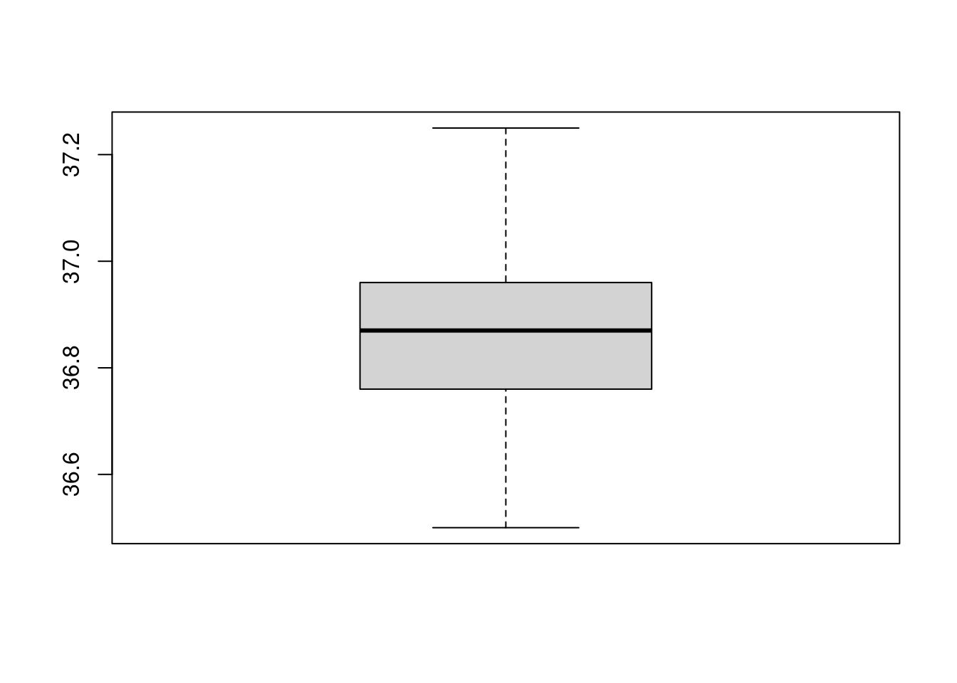
Exercise: Find the formula for the upper and lower
whisker in R.
Another way to look at the distribution of a quantitative variable is
to build its histogram thanks to the hist function:
hist(temp1)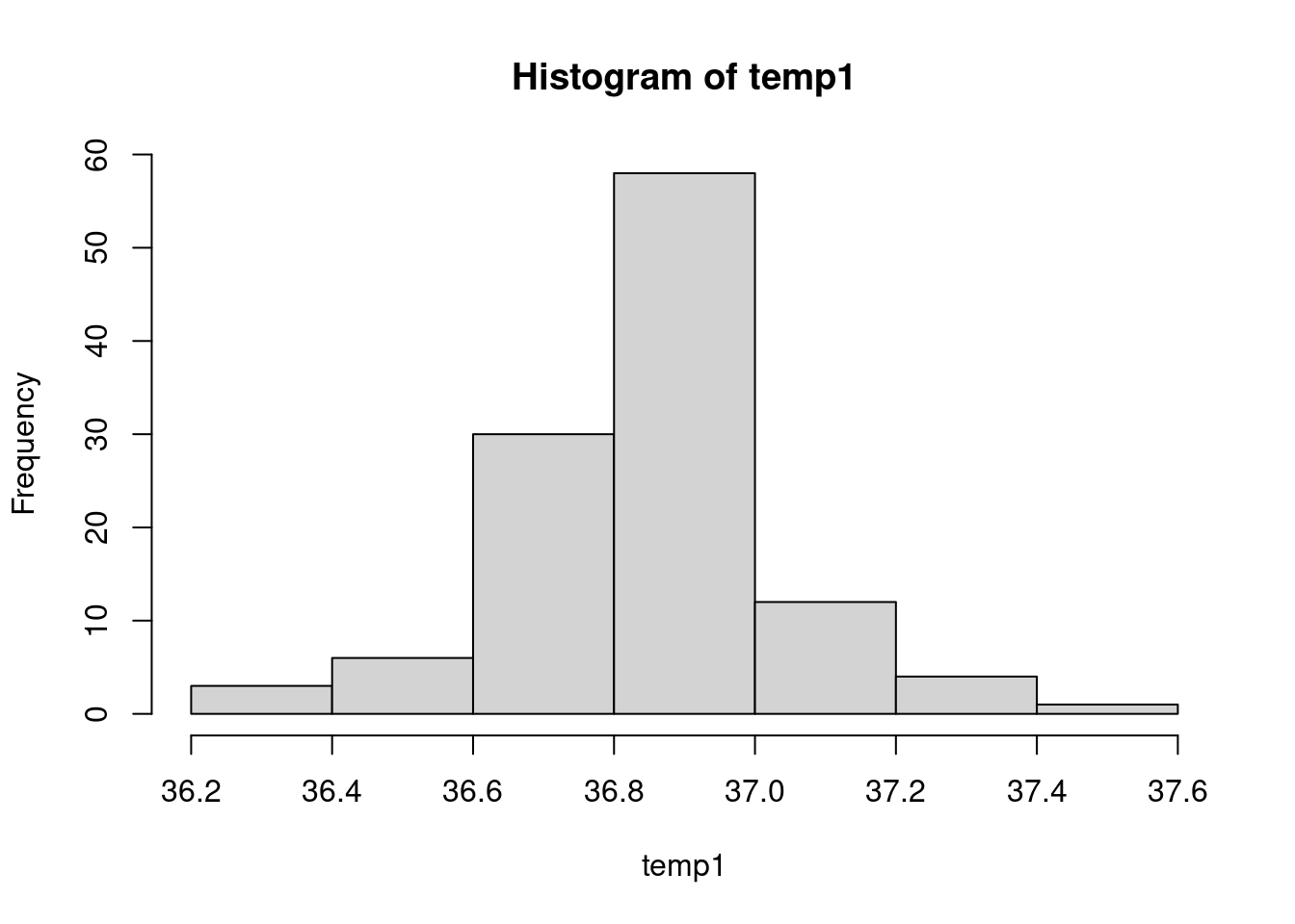
You can choose the number of class with nclass or even
specify each class with breaks. You can also set the
argument freq to false to obtain a histogram where the
total area of the rectangles is equal to 1. This way, the histogram is a
representation of the empirical probability distribution associated to
the data.
hist(temp1, main="My histogram",
     xlab="temperature (Celsius)",freq=F,nclass = 15,
     col="cyan",border = "orange")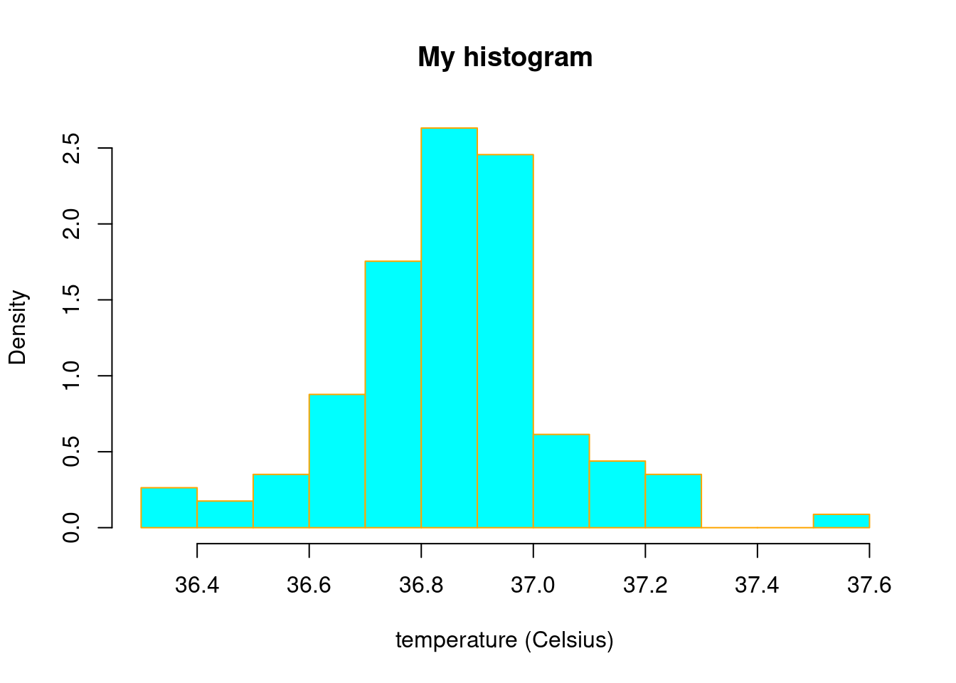
Exercise: Do a histogram of temp1 with
specific breaks.
Variance and standard deviation
Measures of central tendency are complemented by measures of dispersion. The best-known is the variance, which becomes the standard deviation when its root is taken.
The variance is computed thanks to the var function:
var(temp1)## [1] 0.03741196Let us check that this is actually the variance that is computed. Recall the definition of the variance: it is the mean of squared deviations from the mean, that is:
mean((temp1-mean(temp1))^2)## [1] 0.03708379Note the the ^2 squares all the entries in the vector.
The value is not the same !
var(temp1)==mean((temp1-mean(temp1))^2)## [1] FALSEWhy ? In fact, the var function corresponds to the
unbiased estimator of the variance, that is: \[
\frac{1}{n-1}\sum_{i=1}^n(x_i -\bar{x}_n)^2,
\] if \((x_i)_{1\leq i\leq n}\)
is our sample of size \(n\). The biased
version, the one we computed at hand, is \[
\frac{1}{n}\sum_{i=1}^n(x_i -\bar{x}_n)^2.
\] Let us check that it is indeed that:
n=length(temp1)
var(temp1)==(n/(n-1))*mean((temp1-mean(temp1))^2)
## [1] TRUEBy the way, we did our first logical test, thanks to the
== operator.
For the standard deviation, this is the sd function:
sd(temp1)==sqrt(var(temp1))## [1] TRUESo, the sd function used the unbiased version
of the variance.
Go to the next tab !
5. Handling missing values
In the considered data set beaver1, there is no missing
values whereas it is often the case for real data. Let us artificially
introduce missing values for the body temperature in a copy of this data
set:
my_beaver<-beaver1
my_beaver$temp[c(10,45,88)]=NA
my_beaver$temp
## [1] 36.33 36.34 36.35 36.42 36.55 36.69 36.71 36.75 36.81 NA 36.89 36.91 36.85 36.89 36.89
## [16] 36.67 36.50 36.74 36.77 36.76 36.78 36.82 36.89 36.99 36.92 36.99 36.89 36.94 36.92 36.97
## [31] 36.91 36.79 36.77 36.69 36.62 36.54 36.55 36.67 36.69 36.62 36.64 36.59 36.65 36.75 NA
## [46] 36.81 36.87 36.87 36.89 36.94 36.98 36.95 37.00 37.07 37.05 37.00 36.95 37.00 36.94 36.88
## [61] 36.93 36.98 36.97 36.85 36.92 36.99 37.01 37.10 37.09 37.02 36.96 36.84 36.87 36.85 36.85
## [76] 36.87 36.89 36.86 36.91 37.53 37.23 37.20 37.25 37.20 37.21 37.24 37.10 NA 37.18 36.93
## [91] 36.83 36.93 36.83 36.80 36.75 36.71 36.73 36.75 36.72 36.76 36.70 36.82 36.88 36.94 36.79
## [106] 36.78 36.80 36.82 36.84 36.86 36.88 36.93 36.97 37.15Missing values are usually encoded as NA in R, meaning
not available, NA is said to be a logical constant
of length 1 in the help of R. Let us take a look at its algebra:
NA+NA## [1] NA-2*NA## [1] NA1/NA## [1] NAc(1,2)+NA## [1] NA NASo, when attempting to perform an operation with a missing value, it appears that the result is also a missing value (although you need to be cautious when dealing with missing values).
For exemple, when computing the mean:
mean(my_beaver$temp)## [1] NAHopefully, the mean function should have an option that allows to handle missing values:
mean(my_beaver$temp,na.rm=TRUE)## [1] 36.85955The option na.rm=TRUE indicates that the NA
must be removed. Let us check what is indeed computed with this options.
Missing value indices can be obtained as follows:
which(is.na(my_beaver$temp))## [1] 10 45 88The which function gives the TRUE indices
of a logical object, allowing for array indices. Here the logical object
is given through the function is.na indicating TRUE when
the entry is NA and FALSE otherwise. To obtain the vector
without the entries corresponding to the NA we can
type:
without_NA<-my_beaver$temp[-c(10,45,88)]
without_NA
## [1] 36.33 36.34 36.35 36.42 36.55 36.69 36.71 36.75 36.81 36.89 36.91 36.85 36.89 36.89 36.67
## [16] 36.50 36.74 36.77 36.76 36.78 36.82 36.89 36.99 36.92 36.99 36.89 36.94 36.92 36.97 36.91
## [31] 36.79 36.77 36.69 36.62 36.54 36.55 36.67 36.69 36.62 36.64 36.59 36.65 36.75 36.81 36.87
## [46] 36.87 36.89 36.94 36.98 36.95 37.00 37.07 37.05 37.00 36.95 37.00 36.94 36.88 36.93 36.98
## [61] 36.97 36.85 36.92 36.99 37.01 37.10 37.09 37.02 36.96 36.84 36.87 36.85 36.85 36.87 36.89
## [76] 36.86 36.91 37.53 37.23 37.20 37.25 37.20 37.21 37.24 37.10 37.18 36.93 36.83 36.93 36.83
## [91] 36.80 36.75 36.71 36.73 36.75 36.72 36.76 36.70 36.82 36.88 36.94 36.79 36.78 36.80 36.82
## [106] 36.84 36.86 36.88 36.93 36.97 37.15length(without_NA)## [1] 111We have removed the considered indices thanks to
-c(10,45,88) meaning that we want to select all the indices
except (the -) c(10,45,88). Then, we can check
if the two means are equals:
mean(without_NA)## [1] 36.85955mean(without_NA)==mean(my_beaver$temp,na.rm=TRUE)## [1] TRUETwo remarks:
- You can use the abbreviations
TforTRUEandFforFALSE. - In a function, when specifying an argument as here with
na.rm=TRUEit is the operator=which is used, and not the arrow<-.
The var and sd function, as well as other
statistical functions, also have the na.rm option:
var(my_beaver$temp,na.rm=T)## [1] 0.0373498sd(my_beaver$temp,na.rm=T)## [1] 0.193261Exercise: compute the median with missing values.
Go to the next tab !
Simulate random variables
In R, we can not only analyze statistical series but also generate them, including as realizations of (pseudo) random variables.
1. Discrete laws
With a dice
Let us roll a fair dice:
sample(1:6,1)## [1] 5Above, the output of the sample function is a sample of
size 1, which is the second argument, drawn at random from
the set c(1:6), the first argument, which stands for the
set \(\{1,2,3,4,5,6\}\):
1:6## [1] 1 2 3 4 5 6The shortcut 1:6 means “the integers from 1 to 6”. What
if we want a sample of size \(5\) ? We
just change the second armument to \(5\):
sample(1:6,5)## [1] 4 5 3 2 6It seems that the draws are made without replacement. It is clear from:
sample(1:6,7)There is an error saying that we can not have a sample greater than the population size when ‘replace = FALSE’. So, let us try with ‘replace = TRUE’:
sample(1:6,7,replace=T)## [1] 1 6 2 2 3 6 1Here the draws are made with replacement. Let us do a thousand random draws:
#number of draws
n<-1000
draws<-sample(1:6,n,replace=T)
We can look at the barplot of the obtained statistical
series. Do not forget to change the type of the variable !
draws<-as.factor(draws)
plot(draws)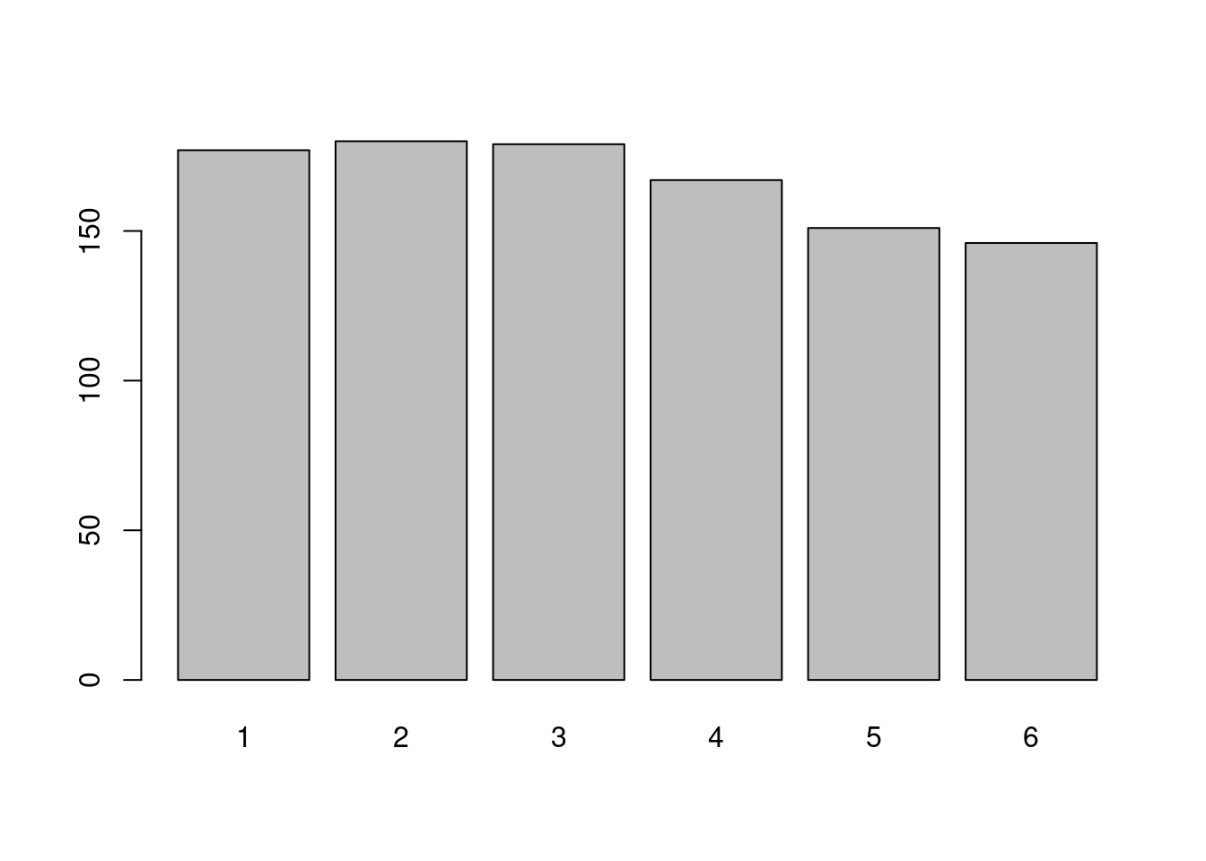
If you do not change the type of the variable, you can also use the
function table, as seen before, together with the
barplot function:
draws<-sample(1:6,n,replace=T)
barplot(table(draws))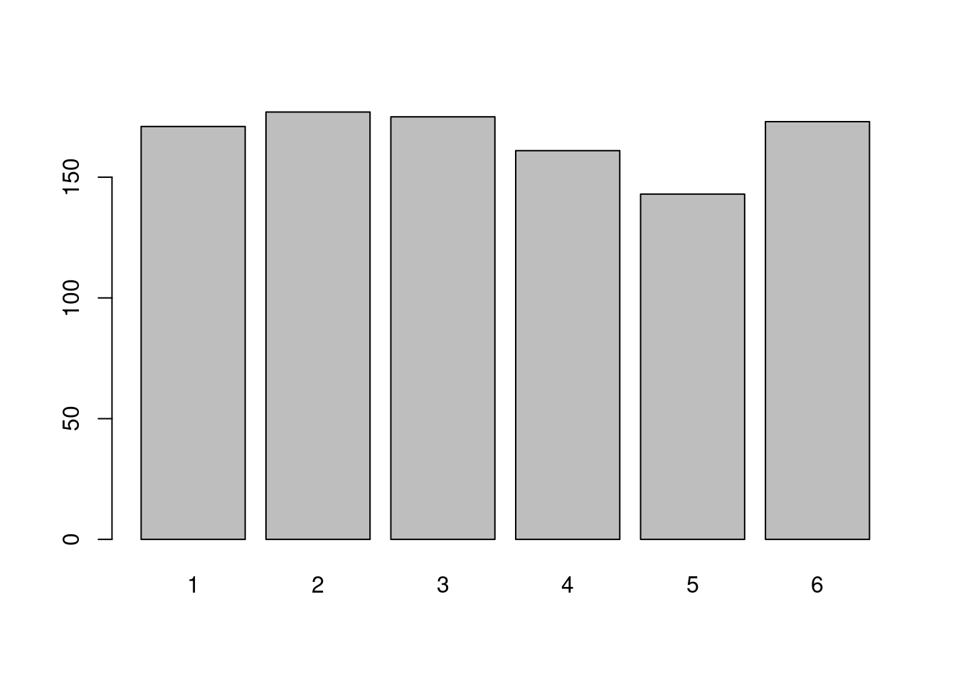
The draws appear to have been made with a fair dice: the frequencies of appearance of each face are very close. This can be changed: you can specify the probability of appearance of each face.
draws<-sample(1:6,n,replace=T,prob = c(4/9,1/9,1/9,1/9,1/9,1/9))
barplot(table(draws))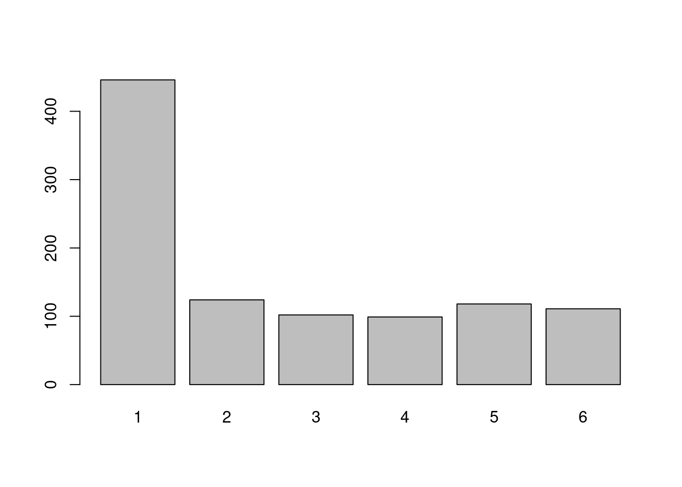
We have changed the probabilities so that the chance to obtain \(1\) is \(4/9\) whereas it is \(1/9\) for the others outcomes. This can be seen on the barplot.
Exercice: Simulate a random variable with values in the integers from \(1\) to \(10\) with associated probabilities proportional to the outcomes.
Standar discrete laws
The binomial law. The binomial distribution models the number of successes when the same experiment is repeated (independently). There is two parameters, \(n\), the number of experiments, and \(p\), the probability of success. Let us write \(X\) a random variable with law the binomial law of parameters \(n\) and \(p\) (we write \(X\sim {\cal B}(n,p)\)).
The acronym in R is binom, with the following syntax for
associated functions:
dbinom(x, size, prob)where thedstands fordensity, in fact here theprobability mass function. The output ofdbinom(x,n,p), for \(x\in\{0,\ldots,n\}\), is \[ \mathbf{P}(X=x)={n\choose x}p^{x}(1-p)^{n-x}. \]pbinom(x, size, prob)where thepstands forprobability, theprobability or cumulative distribution function. The output ofpbinom(x,n,p), for \(x\in\{0,\ldots,n\}\), is \[ \mathbf{P}(X\leq x). \]qbinom(p, size, prob)where theqstands forquantile, thequantile function(a generalized inverse of the cumulative distribution function). The output ofqbinom(p,n,p), for \(p\in(0,1)\), is a \(q\) such that \[ \mathbf{P}(X\leq q)=p. \]- A realisation of \(X\) is given
thanks to
rbinom(k,n,p).
Let us try:
n=10
p=0.8
dbinom(8,n,p)
## [1] 0.3019899choose(n,8)*p^8*(1-p)^(10-8)## [1] 0.3019899pbinom(8,n,p)## [1] 0.6241904sum(choose(n,0:8)*p^(0:8)*(1-p)^(10-0:8))## [1] 0.6241904Note here that we have used the fact that it is possible to pass
vector arguments to certain functions: here for the power
function, the multiplication and the function choose
(binomial coefficient).
Exercise: Find the keyword for the
geometrical law and the Poisson law. Simulate
a sample according to these laws and draw the associated bar chart.
Go to the next tab!
2. A game to learn if and for
Two players roll a dice (one dice per person). If the product of the two outcomes is even, player 1 win, otherwise, it is player 2. What is the probability of each player’s victory?
We do not intend here to compute exactly this probability, but rather to simulate the game and compute an approximation of these probabilities.
Let us play just one time:
D1<-sample(1:6,1)
D2<-sample(1:6,1)
if((D1*D2)%%2==0){
  winner<-1
} else {
  winner<-2
}
winner
## [1] 1Here, we have learned how to test if a condition is satisfied thanks
to the if statement. The syntax is as follows:
if(condition){
  instruction to be done if condition is TRUE
} else{
  instruction to be done if condition is FALSE
}
In the condition, we also used the operator %% which is
the modulo operator: a number is even if it is equal to
\(0\) modulo \(2\).
Now, let us play a thousand of times:
N<-1000
#We play N times
D1<-sample(1:6,N,replace=T)
D2<-sample(1:6,N,replace=T)
#The outcomes
result<-D1*D2
#The winner is the player (1+ the result modulo 2)
winner<-1+(result%%2)
head(winner)
## [1] 2 1 1 1 2 1We can now compute an approximation of the probability of winning for each player:
prop.table(table(winner))## winner
## 1 2
## 0.747 0.253We can show that the probability is in fact \(3/4\) for the player \(1\) (and therefore \(1/4\) for the player \(2\)). What we obtain is quite close due to the law of large number (we will talk about that later).
Exercise: Construct (in R…) an
unbalanced dice such that the probabilities of each player winning are
equal.
Now, still with fair dices, let us assume that if player 2 wins, player 1 gives player 2 €30 and that in the other case, player 2 gives player 1 €\(m\). Can you numerically find \(m\) such that it is a fair game ?
At first, recall that a game is said to be fair if, on average, no money is won or lost. Let us try to form the vector of relative gains when, let say, \(m=3\)€:
m=3
gains=-30*(winner==2)+3*(winner==1)
head(gains)
## [1] -30 3 3 3 -30 3Here we have used a convenient but not sraightforward syntax:
winner is a vector made of 1 and
2, then
head(winner==2)## [1] TRUE FALSE FALSE FALSE TRUE FALSEput FALSE when it is not 2 and
TRUE when it is 2. Then if we multiply this
logical vector by a scalar, TRUE is interpreted as
1 and FALSE as 0 so that since
the multiplication is entrywise:
head(-30*(winner==2))## [1] -30 0 0 0 -30 0We could have done a for loop to obtain the same thing. Let us learn that. At first, we need to declare a vector:
gains<-vector(mode="numeric",length = N)
head(gains)
## [1] 0 0 0 0 0 0It is full of \(0\)… We then put
\(-30\) when the winner is player \(2\) and \(m\) otherwise thanks to a for
loop:
for(i in 1:N){
  if(winner[i]==2){
    gains[i]<- -30
  }else{
    gains[i]<- m
  }
}
head(gains)
## [1] -30 3 3 3 -30 3Note that in R, a vector is indexed from \(1\) (and not \(0\) as in Python).
There is a common alternative to not declare a vector with given
size, it is to use the c function to concatenate or combine
the previous results with the new one. The syntax is as follows:
#A NULL object (or empty)
gains<-c()
for(i in 1:N){
  if(winner[i]==2){
    gains<- c(gains,-30)
  }else{
    gains<- c(gains,m)
  }
}
head(gains)
## [1] -30 3 3 3 -30 3Exercise: Using a for loop on \(m\) from \(0\) to \(10\) by step of \(0.01\), find an approximation of \(m\) such that it is a fair game. To built a
grid you can use the seq function
?seq## [1] 10.17Go to the next tab!
3. Illustration of the law of large numbers and the central limit theorem
A concept often used without necessarily paying attention to it when analyzing data or simulating a random experiment is linked to the frequentist approach to probability, formalized by the law of large numbers.
The law of large numbers states that the average of the results obtained from a large number of independent random samples converges to the true value, if it exists.
We can illustrate this fact. Let us do a large number of independent random experiments (with a dice):
N<-1000
X<-sample(1:6,N,replace=T)
We can compute the running mean a see if it converges towards the true mean, the expectation, wich is \(3,5\) here.
#create a vector of size N full of 0
running_mean<-rep(0,N)
for(i in 1:N){
  running_mean[i]<-mean(X[1:i])
}
We have selected the subset of the values of X from
\(1\) ti \(i\) using the syntax
X[1:i].
We can then plot this running mean to see if it converges towards the true mean:
plot(running_mean,pch=19)
abline(h=3.5,col="red")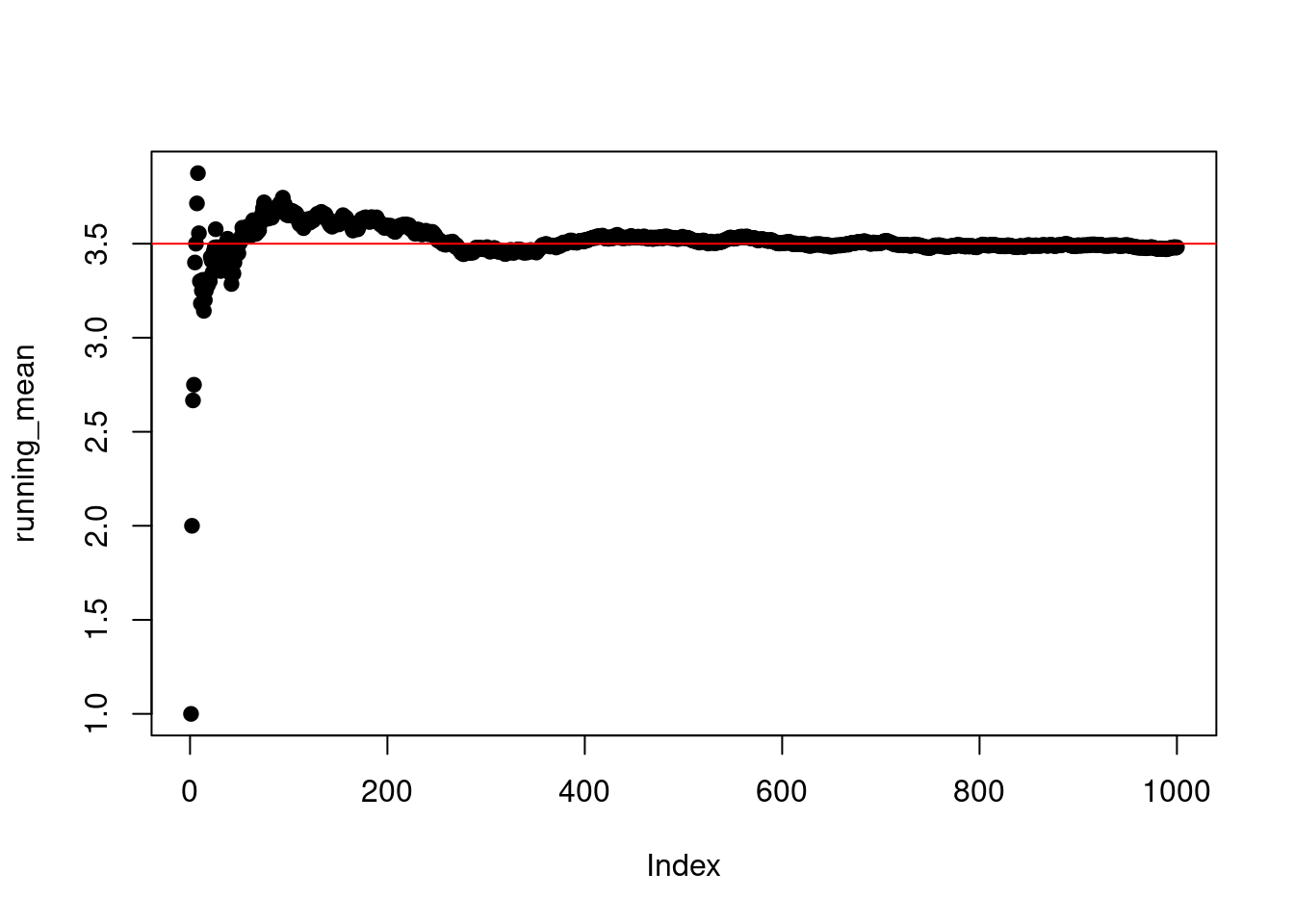
The true value of the mean is represented here by a red horizontal
line obtained using the abline function, which draws
straight lines (here horizontal, thanks to the h argument,
but it’s possible to draw all kinds of lines).
There is shortcuts in R to do loops using the
apply functions. Here with sapply:
running_mean<-sapply(1:N,function(i) mean(X[1:i]))We also could have used the cumsum function here:
running_mean<-cumsum(X)/(1:N)What is remarkable about the law of large numbers is the way it converges. Let us illustrate that by drawing on the same plot the running mean for a hundred of experiments of size \(N=1000\):
plot(0,xlim=c(1,N),ylim=c(2,5))
for(i in 1:100){
  X<-sample(1:6,N,replace=T)
  running_mean<-cumsum(X)/(1:N)
  #We choose a random color
  couleurs<-rgb(runif(1),runif(1),runif(1))
  #and plot the running_mean
  lines(1:N,running_mean,col=couleurs)
}
abline(h=3.5,lwd=1.2,col="red")
We observe that all trajectories enter (with high probability) a certain tube that can be characterized:
plot(0,xlim=c(1,N),ylim=c(2,5))
for(i in 1:100){
  X<-sample(1:6,N,replace=T)
  running_mean<-cumsum(X)/(1:N)
  #We choose a random color
  couleurs<-rgb(runif(1),runif(1),runif(1))
  #and plot the running_mean
  lines(1:N,running_mean,col=couleurs)
}
abline(h=3.5,lwd=1.2,col="red")
lines(1:N,3.5+3*sqrt(35/12)/sqrt(1:N),lwd=1.2)
lines(1:N,3.5-3*sqrt(35/12)/sqrt(1:N),lwd=1.2)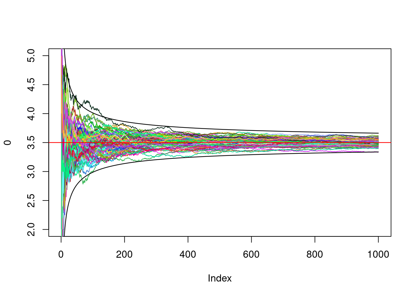
The convergence speed is thus of order \(1/\sqrt{n}\): This is one of the things the central limit theorem tells us. We can also look at the distribution of the ending points:
ending_points<-c()
for(i in 1:1000){
  X<-sample(1:6,N,replace=T)
  running_mean<-cumsum(X)/(1:N)
  ending_points<-c(ending_points,running_mean[N])
}
hist(ending_points,20)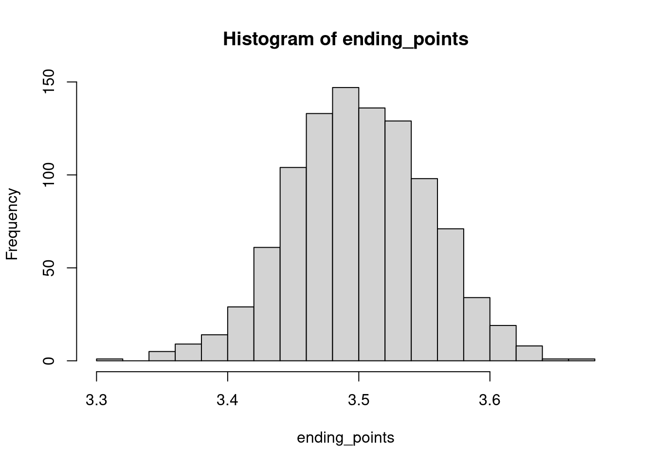
This histogram has the characteristic shape of a bell curve, a shape associated with the normal distribution. Under the right assumptions, the renormalised (by \(\sqrt{n}\)) of the running mean converges, in some sense, towards a normal distribution.
The normal law is a continuous law, see next tab.
4. About continuous laws
The normal law
Roughly speacking, a random variable \(X\) is said to be continuous when the probability that \(X\) belongs to the interval \([a,b]\) can be expressed as an integral \[ \mathbf{P}(X\in[a,b])=\int_a^b f_X(x) dx, \] where \(f_X\) is some positive function, let say piecewise continuous, called the density of \(X\). In statistics, it models what is called a quantitative and continuous variable (when you observe two values, an intermediate value between the two would also make sense).
For the normal law, with parameters \(0\) (the mean) and \(1\) (the variance), the density is \[ x\in\mathbf{R}\mapsto \frac{1}{\sqrt{2\pi}}e^{-\frac12x^2}. \]
Let us simulate a sample of size \(n=1000\) distributed accordind to a normal law with parameters \(0\) and \(1\):
n<-1000
X<-rnorm(n,mean = 0,sd=1)
hist(X,freq=F)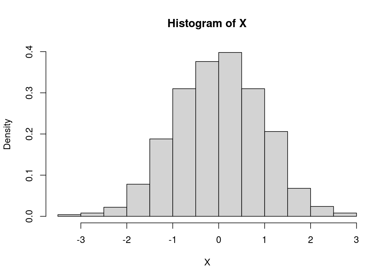
We can show the density graph on the histogram:
n<-1000
X<-rnorm(n,mean = 0,sd=1)
hist(X,freq=F)
x=seq(min(X),max(X),by=0.01)
lines(x,dnorm(x,mean=0,sd=1),col="red",lwd=2)
#verificaton
lines(x,exp(-x^2/2)/sqrt(2*pi),col="blue")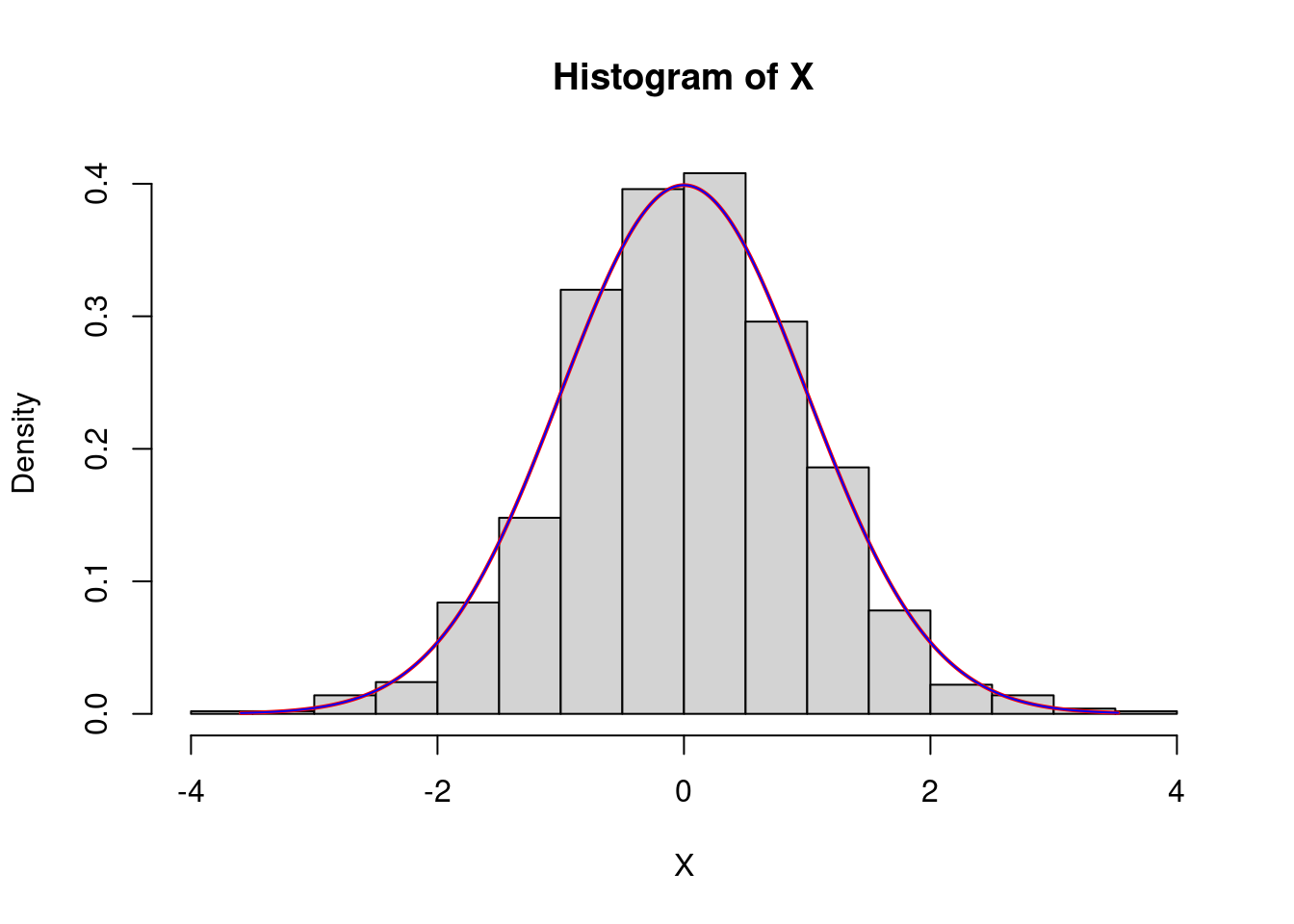
Exercise: Plot the histogram of the square of a normal law with mean \(-2\) and standard deviation \(5\).
The normal law is quite important since it appears in the central limit theorem.
The exponential law
A random variable that follows an exponential law typically models the first time that something occurs (nuclear disintegration, queue areas, cell division…). Its density is : \[ x\in\mathbf{R}\mapsto \left\{\begin{array}{ll}\lambda e^{-\lambda x} \text{ if }x\geq0,\\ 0 \text{ if } x<0, \end{array} \right. \] where \(\lambda\) is some parameter. If \(X\sim\mathcal{E}(\lambda)\), that is if \(X\) follows an exponential law with parameter \(\lambda\), the expectation (or theoretical mean) of \(X\) is \(1/\lambda\). So if \(X\) is in seconds, \(\lambda\) is in hertz, that is it corresponds to a rate or to the mean number of observed phenomena per unit of time.
In R, the keyword is exp:
X<-rexp(1000,rate=2)
mean(X)
## [1] 0.4921805So the rate parameter corresponds to \(\lambda\).
hist(X,freq=F,40)
x<-seq(0,max(X),by=0.1)
lines(x,dexp(x,rate=2),lwd=2,col="red")
#verification
lines(x,2*exp(-2*x))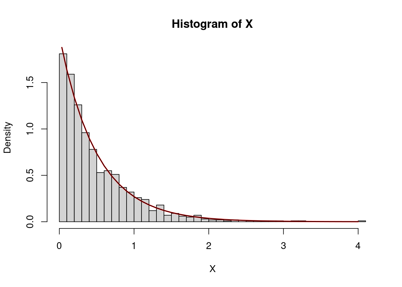
The uniform law
The uniform law on the interval \([a,b]\) with \(a<b\) has for density \[ x\in\mathbf{R}\mapsto \left\{\begin{array}{ll} \frac{1}{b-a} \text{ if }x\in [a,b],\\ 0 \text{ otherwise}. \end{array} \right. \]
In R, the keyword in unif:
U<-runif(1000,min=0,max=1)
mean(U)
## [1] 0.4961109var(U)## [1] 0.08277328Exercise: Using a for loop, find the
integer \(n\) such that the computed
variance of \(U\) is the closest to the
quantity \(1/n\).
Exercise: Try to identify the law of \(\log(U)/3\), where \(U\) follows a uniform law on \([0,1]\).
Exercice: Try to identify the law of \(\sqrt{R}\cos(U)\) where R follows an exponential law with rate \(1/2\) and \(U\) a uniform law on \([0,2\pi]\).