Identification avec scan esacf et minic

1. Simuler un processus ARMA(2,2) suivant
   
   $$X_t = 2.0 + 0.07575X_{t-1}+0.7575X_{t-2} + \varepsilon _t -2.4 \varepsilon _{t-1} + 0.8 \varepsilon _{t-2}$$
   
   
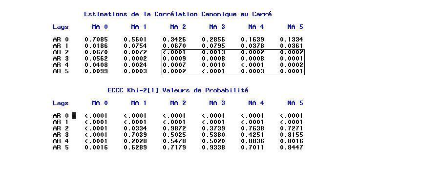
   Utilser la methode scan pour vérifier que le modèle ARMA(2,2) ajuste bien ce processus. Pour comprendre la méthode SCAN on peut lire le manuel de SAS

    
   http://www.math.u-bordeaux1.fr/~hzhang/m2/st/SAS_ETS_ARIMA_SCAN.pdf
   

   Corrigé

    
   /* simulation ARMA(2,2) */
   title1 'Simulated ARMA(2,2)';
   data a; 
        u1=0; u2=0; a1 = 0; a2=0; 
        do i = -50 to 1000; 
           a = 0.2*rannor( 32565 ); 
           u = 2.0+(0.1/1.32)*u1 + (1.0/1.32)*u2 + a - 2.4*a1 + 0.8*a2; 
           if i > 0 then output;  
           u2 = u1; u1 = u; a2 = a1; a1 = a; 
        end; 
   run;
   
   symbol1 interpol=join color=black value=none;
   proc arima data=a;
   	identify var=u scan; run;
   	estimate p=2 q=2 plot method=ML; run;
   quit;
   

   On remarque la zone (rectangle) 0 commence par ARMA(2,2) (ou bien ARMA(3,1))
   

2. Simuler un processus ARMA(1,2) suivant
   
   $$X_t = 2.0 + 0.7575X_{t-1} + \varepsilon _t -2.4 \varepsilon _{t-1} + 0.8 \varepsilon _{t-2}$$
   
   
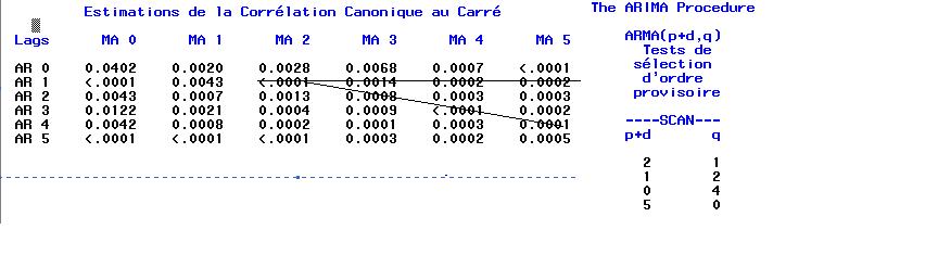
   Utilser la méthode esacf pour vérifier que le modèle ARMA(1,2) ajuste bien ce processus. On peut lire le manuel de SAS

    
   http://www.math.u-bordeaux1.fr/~hzhang/m2/st/SAS_ETS_ARIMA_ESACF.pdf
   

   Corrigé

    
   /* simulation ARMA(1,2) */
   title1 'Simulated ARMA(1,2)';
   data a; 
        u1=0; a1 = 0; a2=0; 
        do i = -50 to 1000; 
           a = 0.2*rannor( 32565 ); 
           u = 2.0+0.7575*u1 + a - 2.4*a1 + 0.8*a2; 
           if i > 0 then output;  
           u1 = u; a2 = a1; a1 = a; 
        end; 
      run;
   
   symbol1 interpol=join color=black value=none;
   
   proc gplot data=a;
   	plot u*i;
   run;
   title1 'identify un arma(1,2) par esacf';
   proc arima data=a;
   	identify var=u scan; run;
   	estimate p=1 q=2 plot method=ML; run;
   quit;
   

   On remarque la zone (triangle) 0 commence par ARMA(2,1), les modèles ARMA(1,2) est acceptable aussi
   

3. Simuler le processus 1, utiliser la méthode SCAN ESACF simultanément pour identify le modèle

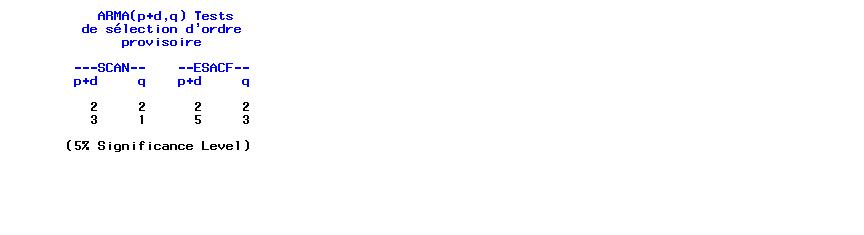
   Corrigé

    
   title1 'identify un arma(2,2) par scan et esacf';
   proc arima data=a;
   	identify var=u scan esacf; run;
   quit;
   

   On remarque que SAS/ETS propose aussi plusieurs modèles, il est raisonable d'utiliser le modèle ARMA(2,2)
   

4. Simuler le processus 1, utiliser la méthode SCAN ESACF MINIC simultanément pour identify le modèle. Le manuel de SAS/ETS pour la méthode MINIC est

    
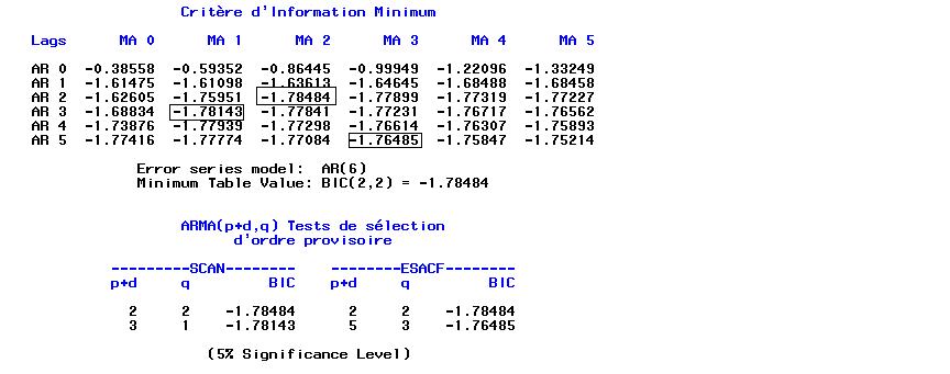
   http://www.math.u-bordeaux1.fr/~hzhang/m2/st/SAS_ETS_ARIMA_MINIC.pdf
   

   Corrigé

    
   title1 'identify un arma(2,2) par scan et esacf';
   proc arima data=a;
   	identify var=u scan esacf minic; run;
   quit;
   

   Plusieurs modèles sont acceptables, il est raisonable d'utiliser le modèle ARMA(2,2), car le BIC (Bayesian information criterion) est minimal.
   
   On peut aussi utiliser une seule option minic.

5. Application : Identifier la serie suivante (Series A de Box Jenkins).

    
   http://www.stat.wisc.edu/~reinsel/bjr-data/index.html
   

   Corrigé

    
   data SeriesA;
   	n=_n_;
   	input x :3.1 @@;
   	datalines;
    17.0 16.6 16.3 16.1 17.1 16.9 16.8 17.4 17.1 17.0 16.7 17.4 17.2 17.4 
    17.4 17.0 17.3 17.2 17.4 16.8 17.1 17.4 17.4 17.5 17.4 17.6 17.4 17.3
    17.0 17.8 17.5 18.1 17.5 17.4 17.4 17.1 17.6 17.7 17.4 17.8 17.6 17.5 
    16.5 17.8 17.3 17.3 17.1 17.4 16.9 17.3 17.6 16.9 16.7 16.8 16.8 17.2 
    16.8 17.6 17.2 16.6 17.1 16.9 16.6 18.0 17.2 17.3 17.0 16.9 17.3 16.8 
    17.3 17.4 17.7 16.8 16.9 17.0 16.9 17.0 16.6 16.7 16.8 16.7 16.4 16.5 
    16.4 16.6 16.5 16.7 16.4 16.4 16.2 16.4 16.3 16.4 17.0 16.9 17.1 17.1
    16.7 16.9 16.5 17.2 16.4 17.0 17.0 16.7 16.2 16.6 16.9 16.5 16.6 16.6 
    17.0 17.1 17.1 16.7 16.8 16.3 16.6 16.8 16.9 17.1 16.8 17.0 17.2 17.3
    17.2 17.3 17.2 17.2 17.5 16.9 16.9 16.9 17.0 16.5 16.7 16.8 16.7 16.7
    16.6 16.5 17.0 16.7 16.7 16.9 17.4 17.1 17.0 16.8 17.2 17.2 17.4 17.2
    16.9 16.8 17.0 17.4 17.2 17.2 17.1 17.1 17.1 17.4 17.2 16.9 16.9 17.0
    16.7 16.9 17.3 17.8 17.8 17.6 17.5 17.0 16.9 17.1 17.2 17.4 17.5 17.9
    17.0 17.0 17.0 17.2 17.3 17.4 17.4 17.0 18.0 18.2 17.6 17.8 17.7 17.2 
   17.4;
   
   symbol1 interpol=join color=black value=none;
   proc gplot data=SeriesA;
   	plot x*n;
   run;
   quit;
   
   proc arima data=SeriesA;
   	/* identify var=x nlag=12 scan;run;*/
   	/* identify var=x esacf; run; */
   	/* identify var=x scan esacf;*/
   	/* identify var=x stationarity=(adf=(5,6,7,8));*/
   	/* identify var=x(1) minic;run;*/
   	identify var=x(1) minic scan esacf; run;
   quit;
   

   Lire le manuel exemple SAS/ETS

    
   http://www.math.u-bordeaux1.fr/~hzhang/m2/st/SAS_ETS_ARIMA_SERIESA.pdf